Quickstart

A labeled kernel is a profile of string lists plus an array. profile reports the numeric shape. labels reports the strings. Label lookup uses the NumPy axis: domain axes first, then codomain axes.

import numpy as np
from fxtensor_salmon import FXTensor

profile = [[["a", "b"]], [["x", "y", "z"]]]
data = np.array(
    [
        [0.1, 0.2, 0.7],
        [0.3, 0.3, 0.4],
    ]
)
tensor = FXTensor(profile, data=data)
assert tensor.profile == [[2], [3]]
assert tensor.labels == ([["a", "b"]], [["x", "y", "z"]])
assert tensor.get_label_index(0, "a") == 0
assert tensor.get_index_label(1, 2) == "z"

The same array can be stored without labels. A tuple (domain, codomain) is also accepted and is always unlabeled.

import numpy as np
from fxtensor_salmon import FXTensor

profile = [[2], [3]]
data = np.array(
    [
        [0.1, 0.2, 0.7],
        [0.3, 0.3, 0.4],
    ]
)
tensor = FXTensor(profile, data=data)
assert tensor.profile == [[2], [3]]
assert tensor.labels == (None, None)

from_strands fills entries from a dictionary. For a labeled profile the keys are nested lists of those labels. Missing keys stay zero.

import numpy as np
from fxtensor_salmon import FXTensor

profile = [[["a", "b"]], [["x", "y", "z"]]]
strands = {
    "[[['a']], [['x']]]": 0.1,
    "[[['a']], [['y']]]": 0.2,
    "[[['a']], [['z']]]": 0.7,
    "[[['b']], [['x']]]": 0.3,
    "[[['b']], [['y']]]": 0.3,
    "[[['b']], [['z']]]": 0.4,
}
tensor = FXTensor.from_strands(profile, strands)
assert tensor.labels == ([["a", "b"]], [["x", "y", "z"]])
assert np.allclose(
    tensor.data,
    [
        [0.1, 0.2, 0.7],
        [0.3, 0.3, 0.4],
    ],
)

Composition

composition is sequential wiring. The codomain of the receiver must equal the domain of the argument. Labels on the result are the receiver’s domain labels and the argument’s codomain labels, and only when both tensors are labeled.

import numpy as np
from fxtensor_salmon import FXTensor

tensor1 = FXTensor(
    [[["a", "b"]], [["x", "y"]]],
    data=np.array(
        [
            [0.2, 0.8],
            [0.6, 0.4],
        ]
    ),
)
tensor2 = FXTensor(
    [[["x", "y"]], [["p", "q"]]],
    data=np.array(
        [
            [0.3, 0.7],
            [0.9, 0.1],
        ]
    ),
)
result = tensor1.composition(tensor2)
assert result.labels == ([["a", "b"]], [["p", "q"]])
assert np.allclose(
    result.data,
    [
        [0.2 * 0.3 + 0.8 * 0.9, 0.2 * 0.7 + 0.8 * 0.1],
        [0.6 * 0.3 + 0.4 * 0.9, 0.6 * 0.7 + 0.4 * 0.1],
    ],
)

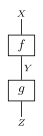
Sequential composition, f ; g.

Tensor product

tensor_product places two morphisms side by side. For states, an empty domain stays empty, so its label group is None.

import numpy as np
from fxtensor_salmon import FXTensor

tensor1 = FXTensor([[], [["a", "b"]]], data=np.array([0.3, 0.7]))
tensor2 = FXTensor([[], [["x", "y", "z"]]], data=np.array([0.2, 0.3, 0.5]))
result = tensor1.tensor_product(tensor2)
assert result.profile == [[], [2, 3]]
assert result.labels == (None, [["a", "b"], ["x", "y", "z"]])
assert np.allclose(result.data, np.outer(np.array([0.3, 0.7]), np.array([0.2, 0.3, 0.5])))

Tensor product, f ⊗ g.

Weather

Labels are arbitrary strings. The same forecast can be named in English or Japanese; only the strings stored on the profile change.

import numpy as np
from fxtensor_salmon import FXTensor

weather_states = ["Sunny", "Rainy"]
sunny_today = FXTensor([[], [weather_states]], data=np.array([1.0, 0.0]))
forecast_matrix = np.array(
    [
        [0.8, 0.2],
        [0.4, 0.6],
    ]
)
forecast_tensor = FXTensor([[weather_states], [weather_states]], data=forecast_matrix)
sunny_tomorrow = sunny_today.composition(forecast_tensor)
sunny_idx = sunny_tomorrow.get_label_index(0, "Sunny")
assert np.isclose(sunny_tomorrow.data[sunny_idx], 0.8)
assert sunny_tomorrow.labels == (None, [["Sunny", "Rainy"]])

import numpy as np
from fxtensor_salmon import FXTensor

weather_states = ["晴れ", "雨"]
sunny_today = FXTensor([[], [weather_states]], data=np.array([1.0, 0.0]))
forecast_matrix = np.array(
    [
        [0.8, 0.2],
        [0.4, 0.6],
    ]
)
forecast_tensor = FXTensor([[weather_states], [weather_states]], data=forecast_matrix)
sunny_tomorrow = sunny_today.composition(forecast_tensor)
sunny_idx = sunny_tomorrow.get_label_index(0, "晴れ")
assert np.isclose(sunny_tomorrow.data[sunny_idx], 0.8)
assert sunny_tomorrow.labels == (None, [["晴れ", "雨"]])

The user guide covers conditioning, Bayesian inversion, copy and discard, and the DisCoPy bridge.